Intro
This is going to be a place where I (slowly) update my data science notes to keep my memory refreshed. I’ve created another Github reporsitory chnynf/data-science-notes to host this markdown file and use Github Actions to automatically push the md file to this post. I’ll be glad if anyone can contribute together to the notes. Most of the snippets here will be the ones I pick up from the internet, from me and my friend’s notes, and from the book All of Statistics: A Concise Course in Statistical Inference, from Larry A. Wasserman.
Random Variables
A random variable is a mapping
Some important discrete random variables
The Point Mass Distribution:
The Discrete Uniform Distribution:
The Bernoulli Distribution:
The probability function is:
The Binomial Distribution:
Flip the coin n times and let X be the number of heads, then
The probability function is:
(Sum of binomials are also binomials.)
The Geometric Distribution:
The number of flips needed until the first heads when flipping a coin:
The probability function is:
The Poisson Distribution:
Count of rare events like radioactive decay and traffic accidents:
The probability function is:
(Sum of Poissons are also Poissons.)
Some important continuous random variables
The Uniform Distribution:
The Normal (Gaussian) Distribution:
The probability function is:
The Exponential Distribution:
Usually used to model the lifetimes of electronic components and the waiting times between rare events:
The probability function is:
The Gamma Distribution:
For alpha > 0, the Gamma function is defined as:
X has a Gamma distribution denoted by:
if:
The exponential distribution is a just a Gamma distribution with alpha equal 1.
The Beta Distribution:
if:
in which Beta function is defined as:
The t and Cauchy Distribution:
if:
The t distribution is similar to a Normal but it has thicker tails. In fact, the Normal corresponds to a t with nu equaling infinity. The Cauchy distribution is a special case of the t distribution corresponding to a t with nu of 1. The density is:
The Chi-Square Distribution:
if:
If Z_1, …, Z_p are independent standard Normal random variables then
Convergence of random variables
Law of Large Numbers:
Sample average converges in probability to the expectation E(X) (average of the population).
Central Limit Therom:
The central limit theorem states that if you have a population with mean μ and standard deviation σ and take sufficiently large random samples from the population with replacement, then the distribution of the sample means converges in distribution to a normal distribution. This will hold true regardless of whether the source population is normal or skewed, provided the sample size is sufficiently large (usually n > 30). If the population is normal, then the theorem holds true even for samples smaller than 30. Sample variance can be calculated as:
Inferences
Point estimation
Point estimation refers to providing a single “best guess” of some quantity of interest.
Let
be n IID data point from some distribution F. A point estimator of a parameter θ is some function of the X’s:
We define bias as the difference between its expectation and θ, and MSE (mean squared error) as:
Confidence Sets
A 1 - α confidence interval for a paramter θ is an interval C_n = (a, b) where a = a(X_1, …, X_n) and b = b(X_1, …, X_n) are functions of the data such that:
Interpretation:
If multiple samples were drawn from the same population and a 95% CI calculated for each sample, we would expect the population mean to be found within 95% of these CIs.
Calculation of normal based confidence interval:
Confidence Interval for Two Independent Samples
In the two independent samples application with a continuous outcome, the parameter of interest is the difference in population means, μ1 - μ2. The point estimate for the difference in population means is the difference in sample means:
If we assume equal variances between groups, we can pool the information on variability (sample variances) to generate an estimate of the population variability:
where:
Then the confidence interval can be calculated as:
or if the sample size is small:
More examples and details:
https://sphweb.bumc.bu.edu/otlt/mph-modules/bs/bs704_confidence_intervals/bs704_confidence_intervals5.html
Hypothesis Testing
Suppose that we partition the parameter space Θ into two disjoint sets Θ0 and Θ1 and that we wish to test:
H0 : θ ∈ Θ0 versus H1 : θ ∈ Θ1
We call H0 the null hypothesis and H1 the alternative hypothesis.
Let X be data and let X be the range of X. We test a hypothesis by finding an
appropriate subset of outcomes R ⊂ X called the rejection region. If X ∈ R we
reject the null hypothesis, otherwise, we do not reject the null hypothesis:
X ∈ R ⇒ reject H0
X ∉ R ⇒ accept H0
Usually the rejection region R is of the form
R = {x ∈ X : T(x) < c}
where T is a test statistic and c is a critical value. The main problem in
hypothesis testing is to find an appropriate test statistic T and an appropriate cutoff value c.
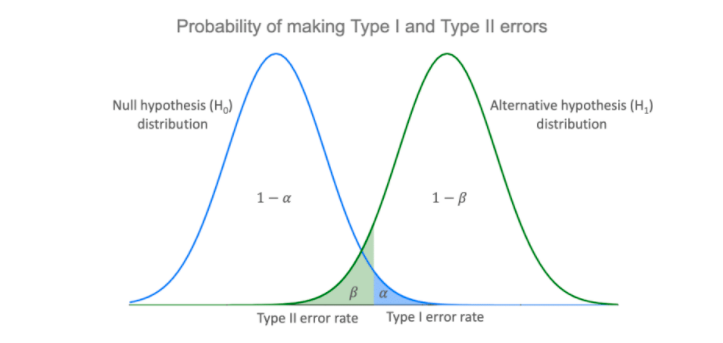
Type I Error and Type II Error
In hypothesis testing, there are two types of errors we can make:
-
Rejecting H0 when H0 is true is called a type I error
-
Accepting H0 when H1 is true is called a type II error
The probability of a type I error is called the significance level of the test
and is denoted by α
- α = P(type I error) = P(Reject H0|H0)
The probability of a type II error is denoted by β
- β = P(type II error) = P(Accept H0|H1)
(1 − β) is called the power of the test
- power = 1 − β = 1 − P(Accept H0|H1) = P(Reject H0|H1)
Thus, the power of the test is the probability of rejecting H0 when it is false.
Simple hypothesis vs composite hypothesis
A hypothesis of the form θ = θ0 is called a simple hypothesis, which corresponds to two-sided tests.
A hypothesis of the form θ > θ0 or θ < θ0 is called a composite hypothesis, which corresponds to one-sided tests.
P-value
The probability of obtaining test results at least as extreme as the results actually observed, under the assumption that the null hypothesis is correct.
Suppose for every α ∈ (0, 1) we have a test of significance level α with rejection
region Rα. Then, the p-value is the smallest significance level at which we can
reject H0:
p-value = inf{α : X ∈ Rα}
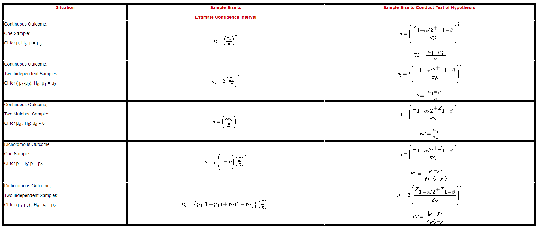
Power and Sample Size Determination
A critically important aspect of any study is determining the appropriate sample size to answer the research question.
The formulas presented here generate estimates of the necessary sample size(s) required based on statistical criteria. (However, in many studies, the sample size is determined by financial or logistical constraints.)
More details at:
https://sphweb.bumc.bu.edu/otlt/mph-modules/bs/bs704_power/BS704_Power_print.html
For confidence intervals
The length of the confidence interval is determined by:
Our goal is to determine the sample size, n, that ensures that the margin of error, “E,” does not exceed a specified value. We can take the formula above and, with some algebra, solve for n:
*Sigma is the population standard deviation, but is estimated based on sample. The unbiased estimation of population variance using sample is calculated as the sum of (x - mean)^2 divided by n-1 instead of n.
In the case of dichotomous outcomes, sigma squared in the above formula can be swapped to p(1-p), which is equal to the variance of a binary vector.
In the case of two samples, referring to the formulas above in the Confidence Interval for Two Independent Samples. A similar formula to calculate n can be derived.
For hypothesis testing
In hypothesis testing, because we purposely select a small value for α , we control the probability of committing a Type I error. The second type of error is called a Type II error and it is defined as the probability we do not reject H0 when it is false. The probability of a Type II error is denoted β , and β =P(Type II error) = P(Do not Reject H0 | H0 is false). In hypothesis testing, we usually focus on power, which is defined as the probability that we reject H0 when it is false, i.e., power = 1- β = P(Reject H0 | H0 is false). Power is the probability that a test correctly rejects a false null hypothesis. A good test is one with low probability of committing a Type I error (i.e., small α ) and high power (i.e., small β, high power).
Here we present formulas to determine the sample size required to ensure that a test has high power. The sample size computations depend on the level of significance, α, the desired power of the test (equivalent to 1-β), the variability of the outcome, and the effect size. The effect size is the difference in the parameter of interest that represents a clinically meaningful difference. Similar to the margin of error in confidence interval applications, the effect size is determined based on clinical or practical criteria and not statistical criteria.
In studies where the plan is to perform a test of hypothesis comparing the mean of a continuous outcome variable in a single population to a known mean, the hypotheses of interest are:
H0: μ = μ 0 and H1: μ ≠ μ 0 where μ 0 is the known mean (e.g., a historical control). The formula for determining sample size to ensure that the test has a specified power is given below:
Here ES is called the effective size, and it’s calculated as:
where μ 0 is the mean under H0, μ 1 is the mean under H1 and σ is the standard deviation of the outcome of interest.
In the case of dichotomous outcomes, p would effectively be the means, and variance is basically p(1-p). So ES can be calculated as:
In the case of two independent samples of continuous outcomes:
*n is the sample size of each group, not combined.
Recall that in the ES calculation, σ is the standard deviation of the outcome of interest. If data are available on variability of the outcome in each comparison group, a pooled estimate of the common standard deviation can be calculated as:
Summary
Machine Learning and Deep Learning
Activation Functions
Sigmoid
- 0 to 1
- Lose gradient at both ends
- Computation is exponential term
Tanh
- -1 to 1 (centered at 0)
- Lose gradient at both ends
- Still computationally heavy
ReLU
- No saturation on positive end
- Can cause dead neuron (if x <= 0)
- Cheap to compute
Leaky ReLU
- Learnable parameter
- No saturation
- No dead neuron
- Still cheap to compute
*No one activation is best. ReLU is typical starting point. Sigmoid is typically avoided in deep learning due to the computation cost.
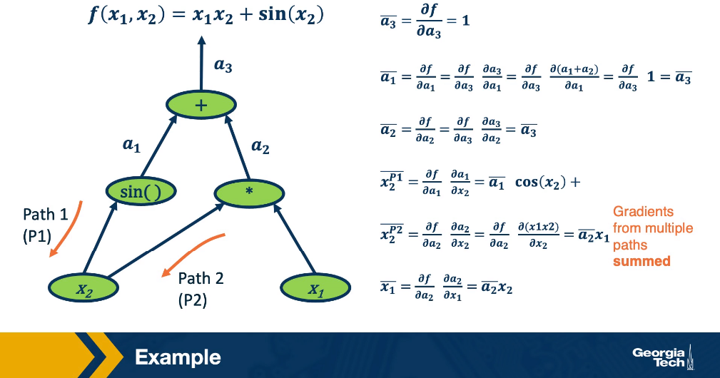
Back Propagation
Initialization
Ideally, we’d like to maintain the variance at the output to be similar
to that of input.
Xavier Initialization
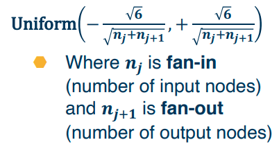
In practice, simpler versions perform empirically well:
For tanh or similar activations:
For ReLu activations:
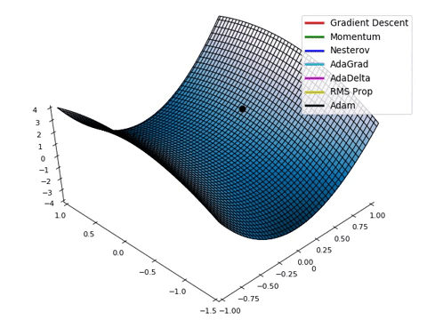
Optimizers
Regularization
L1
*Better for feature selection.
L2
Dropout Regularization
For each node, keep its output with probability p; Activations of deactivated nodes are essentially zero. During testing, no nodes are dropped. During test time, scale outputs (or equivalently weights) by p, so that train and test-time input/output can have similar distributions.
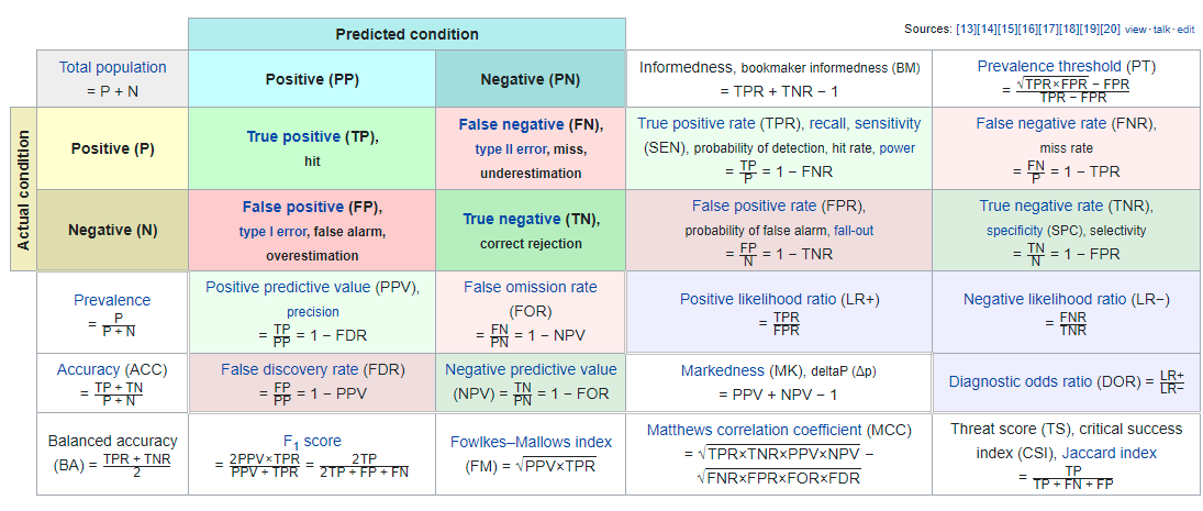
Evaluation
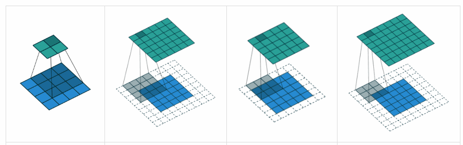
Sizes of convolution and pooling layer outputs
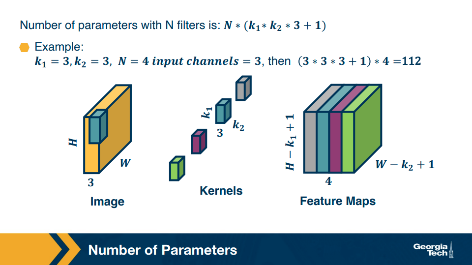
- Valid convolution – no padding
- Same convolution – enough padding added maintain same input and output size
- Full convolution – enough zeros are added for every pixel to be visited k times in each direction, resulting in an output image of width m + k − 1
Miscellaneous
Statistics / Data Mining Dictionary
| Statistics | Computer Science | Meaning |
|---|---|---|
| estimation | learning | using data to estimate an unknown quantity |
| classification | supervised learning | predicting a discrete Y from |
| clustering | unsupervised learning | putting data into groups |
| data | sample | |
| covariates | features | the |
| classifier | hypothesis | a map from covariates to outcomes |
| hypothesis | subset of a parameter space |
|
| confidence interval | interval that contains unknown quantity with a predicted frequency | |
| directed acyclic graph | Bayes net | multivariate distribution with specified conditional independence relations |
| Bayesian inference | Bayesian inference | statistical methods for using data to update subjective beliefs |
| frequentist inference | statistical methods for producing point estimates and confidence intervals with guarantees on frequency behavior | |
| large deviation bounds | PAC learning | uniform bounds on probability of errors |
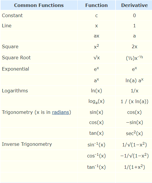
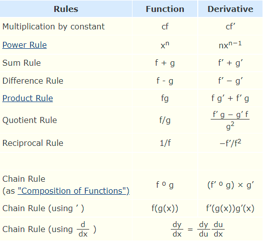
Common Derivatives